Conditional Formatting - Duplicates

Before any mailing goes out the door, your constituent list deserves a quick health check. Duplicate records in a direct mailing mean duplicate postage. A stray space can break a mail merge. A misspelled salutation can land in front of your biggest donor. The good news: Excel's Conditional Formatting can spotlight all of these problems in seconds with no formulas buried in helper columns, no add-ins, just color.

In the lesson below, you will learn how to use the tool to identify duplicates with a simple example. To learn how to use Conditional Formatting on a more complex direct mail list, register for our free webinar on Thursday, August 13 at 3pm EST.

• Select the column most likely to be unique, usually the account or constituent ID. If you are pulling a list from your own CRM, ALWAYS include that ID. If you are working from an outside list, the most likely unique field will be Email. For this example, that’s the field we’ll use.

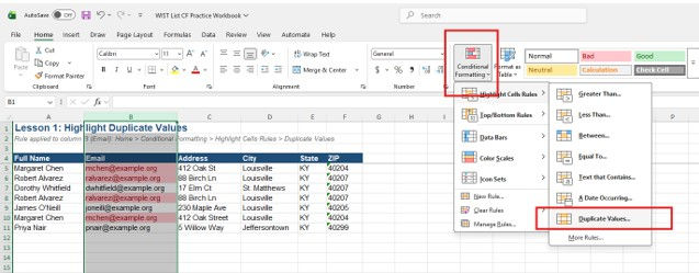
• Highlight the column containing the email.

• Go to Home > Conditional Formatting > Highlight Cells Rules > Duplicate Values

• Keep the default red fill and click OK. Every value that appears more than once lights up.

  
  

  

  
  

• At this point, it’s helpful to sort your entire sheet on the Email column.

  
  

  

  
  

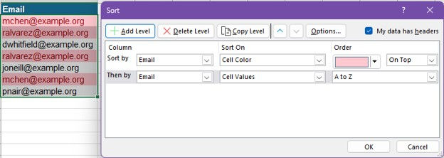
• Sort by color first, with the pink on top. The sort by the email itself. Then you will see all the duplicates next to one another.

• Now you can delete the rows you want to ignore.

If you find records that have the same email, but have different names or addresses, you will have to make choices about what is correct. Whatever you decide, make the changes in your CRM, not just the list! Your future self will thank you.

Now that you know the basics of Conditional Formatting, you might find other uses for it to help with your data hygiene. For a tutorial on how to use the tool for a more complex direct mail list, don’t forget to register for our free webinar.